Vortex dipoles by PIV method
Click here to see the images and the short movies from this lab
Introduction
A vortex dipole is a jet flow with a system of two vortices of opposite sign at its front. Vortex dipoles are widespread in the ocean and are often observed in satellite images of the ocean surface (Figure.1).
Figure 1. Satellite image of the Black Sea. Vortex
dipole formed by cold water (dark) is clearly visible in the central part of
the sea.
Vortex dipole performs translational motion and can therefore be characterized by its net linear momentum. Thus the generation of dipoles requires the action of a force on a fluid.
In the ocean the wind can often apply such a localized force on the ocean surface. Another essential condition is required for generation of dipoles: the flow must be planar. Dipoles easily occur in a density stratified (layered) fluid where the gravitational force suppresses vertical motion. To make the current visible some indicator (passive tracer) is usually needed. In the ocean it is usually a temperature contrast. In the lab we use dye to make the flow visible.
The maximum cross-correlation (MCC) method is a procedure for reconstructing velocity field in the flow. In this procedure, the displacements of small regions of the patterns of passive tracer are estimated between sequential images using cross-correlations between small rectangular sections from each image. This technique is widely used in experimental fluid dynamics (see e.g. [1]). The approach called Particle Imaging Velocimetry (PIV) is commonly used when small particles of neutral density are seeded in the fluid. We will use small (50 mm) plastic spheres of almost the same density as water.
Experiment
1.Creation of density stratification.
The simplest case of stratification is a two-layer system. A Plexiglas tank is filled with two layers of fluid of different densities. The lower layer can be relatively thick, 2-3 cm, and consists of heavy fluid: salt water with a concentration of salt 50-100 g per litre of water. The upper layer should be as thin as possible, 0.3-0.5 cm, and consists of a light fluid: fresh water. To prepare a two-layer system without mixing the fluids, one can float a sheet of paper on top of the salt water. The fresh water is carefully poured onto the sheet, and the latter is then (very carefully) removed.
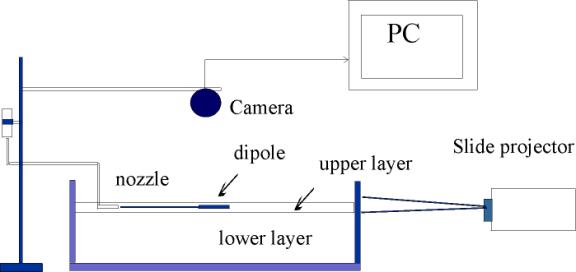
Figure 2. Experimental set-up.
2.Observation of vortex dipoles
Place the nozzle (epidermic needle) in the upper layer as shown in fig.2. Use dyed fresh water (provided) to generate a horizontal jet flow from the nozzle. This submerged jet is used to reproduce the action of a localized force on the fluid. Observe the development of the vortex dipole. By lowering and raising the burette, one can vary the difference Dh between the water level in the tank and that in the burette and thereby vary the intensity of flow from the nozzle. Adjust the height of the burette so that the flow is laminar (the dipole is well formed). Record a 1min long movie using the camera (put the transparent ruler under the tank, start the camera before you start the flow, use the frame rate of 2 frames per second). Repeat the experiment (without recording) to measure the time required for the level of water in the burette to fall at certain value (e.g. 0.5 or 1.0 ml). Note that the level of water in the burette should not change too much since we would like to keep Dh almost constant for the intensity of the flow from the nozzle to be constant. The ratio of this volume to the measured time interval gives you the mean volume flux rate, q, during the experiment.
Using the “Intel Create & Share” software to look through the recorded movie and
to save single frames.
- Find a frame which corresponds to the start of the flow from the nozzle. Make note of the number of this frame.
- Save 5-10 consecutive frames which cover the full range of translation of the dipole. Make notes of the frames numbers.
The files will be saved in the directory C:\Galleries\Flow_image. Start Windows Explorer from the Start menu. Double clicking on the files in the Windows Explorer will allow you to see the saved frames in the Paint (Windows image tool). Use the cursor to measure the length L and width D of the dipole (see Figure 3) for different frames (the position of cursor in pixels is shown by Paint). Use one of the images with the ruler to determine the resolution of your images (in pixels per cm). You will need this value later for PIV analysis.
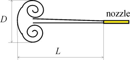
Figure 3. Sketch of the vortex dipole
3.PIV
Discard the fluid in the tank and create the stratification again. This time use water with seeding particles (provided) for the upper layer. Use fresh water (no particles) for the nozzle. Before filling the tank put black paper under the tank. Switch on the slide projector and direct the beam to the side of the tank. Fix two stripes of black paper on the side of the tank to make a slit so that only the interface between the layers and upper layer are illuminated. To obtain good quality images it is important to cut the extra light so that neither the surface of water or bottom of the tank are illuminated. Remember that if you are able to see the flow clearly by eye then the camera will probably see it too. Record 1 min movie using the frame rate of 4 frames per second. Note that the video files are very large in size (50-80 Mb), try to cut unnecessary recording time. Using the “Intel Create & Share” software save two successive
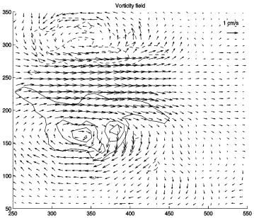
Figure 4. Velocity (arrows) and vorticity (contours) in the dipole.
frames from the recorded movie (choose the frames where the motion of particles show the flow in the dipole most clearly). Sometimes, bottlenecks occur in transferring data to the hard disk of your computer during the recording so that frames are dropped. Choose only those consecutive frames where you are able to see the displacements of particles between the frames.
Use the Partim software to reconstruct the velocity, v, and vorticity, w=curl v, fields (see example in Figure 4).
4.Data analyses
Plot the graphs of L and D versus time (use the frames numbers to calculate time). Implying that the flow is governed mainly by the viscous force (i.e. L and D depend only on the coefficient of kinematic viscosity, n (cm2/s) and time, t) estimate the time dependence of L and D using the dimensional analysis. Do the results of your measurements agree with this estimate?
Previous experiments [2] show that dipoles develop self-similarly. (If the distributions of quantities characterizing some physical process are similar at different times, such a process is called self-similar). For this particular flow this means that D is proportional to L, D = aL, the coefficient of proportionality a being the function of a nondimensional parameter called the Reynolds number. The Reynolds number, Re, represents the ratio of inertial forces to viscous forces. At high values of Re the flow experiences a transition from laminar to a turbulent regime. The coefficient a is plotted in Figure 5 as a function of Re2. Using your experimental data estimate the value of a and find the value of the Reynolds number from the plot in Figure 5.
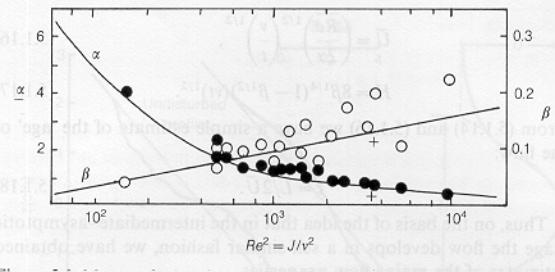
Figure 5. a for different values of the Reynolds number.
The Reynolds number can be also estimated via the momentum flux rate, rJ from the nozzle. A jet from a round nozzle (measure the internal diameter d of the nozzle using the microscope) is injected into surrounding fluid. If the mean velocity at the nozzle exit is U then the mass flux rq (q is the volume flux you measured in the experiment and r = 1g/cm3 is the density of water) is proportional to q = p d2U/4. The injected fluid transports momentum, the momentum flux rJ being proportional to
J = p d2U2/4 = 4q2/(p d2).
According to Newton’s second law of motion, the rate of
change of the momentum of the system is equal to the magnitude of the force
applied. Thus the source acts on the fluid with a total force F = rJ. The value of J can be
nondimensionalized by n2 (for
water n = 0.01 cm2/s) . It
is shown in [2] that Re2 = J/n2. Calculate the value of Re and
compare it with that obtained from the graph. What is the value of force F in Newtons?
Partim calculates two components of velocity VXi and VYi and vorticity field OM represented by arrays in Matlab code. These arrays are kept in memory. You can use them for further analysis writing simple Matlab commands.
- Verify that the total vorticity in the flow is almost zero (sum all of the elements of the array OM, compare the result with a sum of only the positive elements of the array).). For example, to sum the positive elements of the two-dimensional array OM you can use the following Matlab command: sum(sum(OM.*(OM>0)))
- Estimate the x and y components of the total momentum of the flow (sum the elements of the arrays VXi and VYi ). This gives you the mometum per unit height of the upper layer of fluid. How is the total momentum related to the momentum flux J?
References:
- A.M.Fincham and G.R.Spedding. Low cost, high resolution DPIV for measurement of turbulent fluid flow. Exp. in Fluids, 23, 449-462
- S.I.Voropayev and Ya.D.Afanasyev. Vortex Structures in a Stratified Fluid: Order from Chaos. Chapman and Hall. London 1994.
Appendix A: Video camera control
Start “Life View USB Robocam” from the Start menu (or click
the icon on the Desktop). Wait until you see the picture in the window. Click
the first icon (Options), go to Video Format, set resolution to 640x450, color
depth 12, click OK. Click the first icon again, go to Capture Setting set the
frame rate to 2 frames per second for the part 2 of the experiment or to 4
frames per second for the part 3 (PIV), enable time limit (60 s), click OK. To adjust the brightness of the picture
if needed click the first icon, go to Video Source, adjust exposure. To record the video click the second icon
(you may need also to click it again to stop the recording), save the files in
the directory C:\Galleries\Flow_image so that they will be easily
accessible by “Intel Create & Share” software.
Appendix B: Looking through AVI movies and saving frames.
Start the “Intel Create & Share” software, click File then Add File to Gallery. Add your saved movie Live#.avi from the directory C:\Galleries\Flow_image to gallery. Double click on the icon in the Gallery to see the movie. Choose the best frames, save the frame clicking the Save Frame button, then click once on the right arrow to move to the next consecutive frame and save it. Remember the names of the files you just saved.
Appendix C: Running Partim.
Open Matlab window. Type the command: PIVmain (to run Partim software). At the prompt, enter the names of the 2 consecutive frames saved previously. Enter the resolution of your image (calculated in part 2) and the frame rate used to record the movie.